Matrices operations calculator

Operations on two matrices

Matrix A

Scalar multiply:

Determinant:
Rank:
Trace:

Matrix B

Scalar multiply:

Determinant:
Rank:
Trace:

Result Matrix C

Scalar multiply:

Determinant:
Rank:
Trace:

Types Addition Determinants Transposed Inverse Rank Scaling

Rotation Eigenvalues

Calculator notes:

1) Operations on matrices A anb B are denoted by highlighting the operation button [+] [−] or [X] by bold green.

2) Any operation done on matrix C will disconnect the operation button to indicate that matrix C is no longer a result of an operation on matrices A and B.

3) Calculations like: 2A^-1 + 3B^T can be performed easily, it is possible to extend the calculation capabilities by the copy operation.

4) The arithmetic buttons are enabled to indicate the allowed operations according to the sizes of the matrices.

Example: Find the value of the expression A² − 4A − 5 I.

if A =

1	2
3	4

Solution

Step 1: Enter matrix A values.

Step 2: Copy matrix A to matrix B.

Step 3: Press on matrix A square button A².

Step 4: Enter the value 4 into scalar multiply of matrix B.

Step 5: Press on the minus button.

Step 6: Copy the result of matrix C into matrix A.

Step 7: At matrix B update the scalar multiply to 1.

Step 8: At matrix B press the unit I matrix button.

Step 9: At matrix B enter the value 5 in the scalar multiply.

Step 10: Because the minus button is already illuminated by the last operation, table C contains the final answer.

-2	2
3	1

Matrices overview

The notation of a matrix of size (m ✕ n) is defined as A(m ✕ n) = A(rows, columns)

A convenient shorthand which offers considerable advantage when working with system of linear equations is by using the matrix notation. Consider the set of linear equations of the form:

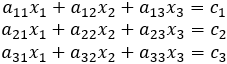
In matrix notation these equations may be represented as:

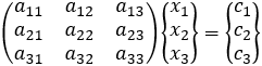
or AX = C

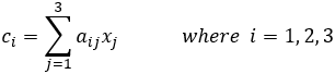
The terms of the matrix can be represented as:

Distributive law

Left side A(B + C) = AB + AC

Right side (A + B)C = AC + BC

A(m ✕ n) B and C (n ✕ p)

A and B (m ✕ n) C(n ✕ p)

Associative law

Addition (A + B) + C = A + (B + C)

Multiplication (AB)C = A(BC)

(m ✕ n)

(n ✕ n)

Scalar multiplication

(kA)B = A(kB) = k(AB)

A(m ✕ n) B(n ✕ p)
k any number

Commutative law

Addition A + B = B + A

Multiplication not commutative

A and B (m ✕ n)

Because A∙B ≠ B∙A

Other algebraic laws

(k, v are constants)

0 + A = A k(A + B)= kA + kB

1 · A = A (k + v)A = kA + vA

0 · A = 0 k(vA) = (kv)A

A + (−A) = 0 kA = 0 → k = 0 or A = 0

(−1)A =  A

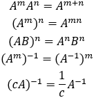
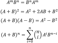
Matrices powers

(c is constant)

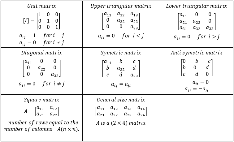
Matrices Types

Matrices addition and multiplication

Matrices addition: A and B are of the same size m × n

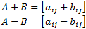
Scalar multiplication:

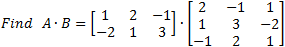
Matrices multiplication A (m × n) ∙ B (n × p) = C (m × p)

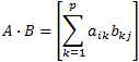
Example:

Determinants

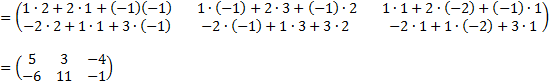
Determinants - symbol: det A or |A|

The result of the determinant of a matrix (n ⨯ n) is a real number.

Size 2 matrix

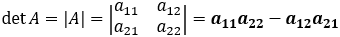
Size 3 matrix

General form to evaluate determinant values:

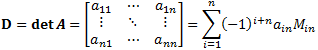
In this formula M_in is the determinant of the submatrix of A obtained by deleting its ith row and nth column. The determinant M_in is called the minor of the element a_in and his size
is (n-1) ⨯ (n-1).

Cofactors of matrix A_ij

It is convenient to consolidate the quantity (-1)^i+j and the minor M_ij . We define the cofactor A_ij of the element a_ij in determinant A as: A_ij = (-1)^i+jM_ij

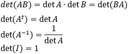
Determinant’s properties:

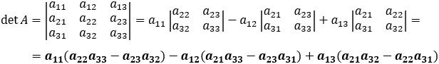
Example: Find the value of the determinant:

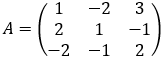
det A = 1 (1 * 2 − (- 1)(- 1))-(-2)(2 * 2 - (-1)(-2)) + 3 (2 * (-1) - 1 * (-2))

det A = 1 (2 − 1) + 2 (4 − 2) + 3 (− 2 + 2) = 5

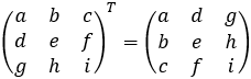
Transposed matrix A^T

Transposed matrix A^T
Interchange of terms across the main diagonal

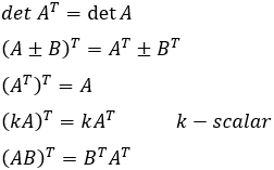
Transposed matrices properties:

Example:
Find the transposed of the matrix.

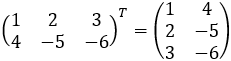
Note: The transposed size of an m ⨯ n matrix is n ⨯ m.

Inverse matrix A^-1

Inverse matrix A^-1 = B

The matrix A is inversible if there is a matrix B so that:
AB = BA = I then the matrix B is the inversed matrix of A.
Matrix I is the unit matrix. Thus the solution of A X = B can be written in the form X = A^-1 B (where A is an n x n matrix and X and B are n x 1 matrices).

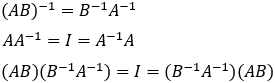
Inversed matrices properties:

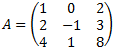
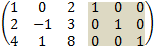
Example: Find the inverse of matrix A

1. Add the unit matrix at the right:

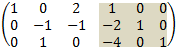
2. Multiply first row by -2 and add it to the second row then multiply first row by -4 and add it to the third row to obtain:

3. Add second and third rows to obtain:

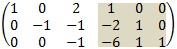
4. Subtract third row from second row:

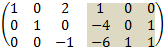
5. Finally multiply third row by 2 and add it to the first row and multiply third row by -1 to get the unit matrix:

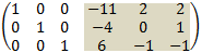
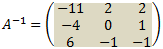
And the inverse of A is:

Rank of a matrix A

Rank of matrix A

A square matrix is said to be non-singular, if its determinant is not zero. The rank of an m ⨯ n matrix is the largest integer r for which a non-singular r ⨯ r submatrix exists. If A and B are an n ⨯ n matrices then: rank(A + B) ≤ rank A + rank B

Example: Find the rank of matrix A (4X3).

1. Multiply first row by 2 and add it to the second row.
2. Multiply first row by -3 and add it to the third row.
3. Subtract fourth row from the first row to get:

4. Add second row to the third row.
5. Subtract fourth row from second row to obtain:

6. Add 2nd row to the 3rd row.
7. Add 3rd row to the 4th row to get:

8. Remove the all 0 row to get the final 3 X 3 matrix.

And the rank of matrix A is 3.

Scaling Matrices

Enlarging or shrinking a vector can be done by multiplying the vector by the diagonal matrix of the form:

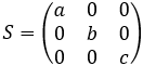
If a = b = c > 1

Then the vector is enlarging equally in all directions.

If a = b = c < 1

Then the vector is shrinking equally in all directions.

If a ≠ b ≠ c

Then the vector is scaling in different sizes in the x, y and z directions.

Eigenvalues and eigenvectors

The system (λI − A) = 0 has a non trivial solution if and only if det |λI − A| = 0. If P denote the matrix of the eigenvectors and B denote the diagonal matrix with diagonal elements being the eigenvalues λ_i of A.

We can write:	AP = PB
	P^{− 1} AP = B or A = PBP^{− 1}

In this case, A is said to be similar to B.

Example: Find the eigenvalues and the eigenvectors of the matrix A =

From the eigenvalues equation we get the characteristic polynomial:

The eigenvalues are the roots of the characteristic polynomial, and are: − 2, − 2, 4 this values are the diagonal values and has the same determinant value as matrix A. In order to find the eigenvectors, substitute first solution λ =− 2 into the characteristic matrix, the result is:

Those equations reduce to one independent equation:	x − y + z = 0
Choose arbitrary y = 0 to receive the first eigenvector	x = 1, y = 0, z = − 1
Choose arbitrary z = 0 to get the second vector:	x = 1, y = 1, z = 0

Perform the same process with the third solution λ = 4 to get:

The result is two independent equations:	x + y − z = 0 and 2y − z = 0
Choose arbitrary y = 1 to receive the vector	x = 1, y = 1, z = 2

The three eigenvectors are:

We can see that the result is matching to the definition of the eigenvectors and eigenvalues:

Rotation Matrices

Rotation of a vector is performed by applying the rotation matrix R on the vector V. V^' = R × V

If the rows and columns of a rotation matrix R are orthogonal to each other and of unit length then the following relations are true:

R^T = R^{− 1} R^T R = RR^T = I detR = 1

Two-dimensional rotation

Rotation by θ counterclockwise

+θ counterclockwise
−θ clockwise

Rotation by θ clockwise

sin(−θ) = −sinθ
cos(−θ) = cosθ

Rotation by 90° counterclockwise

Rotation by 180° counterclockwise

Rotation by 270° counterclockwise

Three dimensional rotation (θ − x axis, ϕ − y axis, φ − z axis)

Rotation about
x axis

Rotation about>
y axis

Rotation about
z axis

Combined rotation in the direction of all axes can be done by multiplying the three rotation matrices in the x,y and z direction

Counterclockwise:	R_xyz = R_x(θ)∙R_y(ϕ)∙R_z(φ)
Mixed direction:	R_xyz = R_x(−θ)∙R_y(−ϕ)∙R_z(φ)

Rotation in the direction of two axes can be done by:

R_xy = R_x R_y

R_xz = R_x R_z

R_yz = R_y R_z

clockwise rotation matrix of the axes (vector is moved counterclockwise)
Note: the order of the rotation is important as rotation R_x (θ) R_y (ϕ) R_z (φ) is not equal to rotation
R_z (φ) R_y (ϕ) R_x (θ).

Counterclockwise rotation matrix of the axes (vector is moved clockwise)

Example:
Rotate the vector V = 2i + j

by 30° counterclockwise.

(Rotated vector) V ^' = R × V (R - Rotation matrix)

V^' = [2 cos(30°) − sin(30°)]i + [2 sin(30°) + cos(30°)]j
V^' = 1.23i + 1.87j

Example:
Rotate the vector V = i + j + k by an angle of 30° counterclockwise about the x axis, 45° clockwise about the y axis and 60° clockwise about z axis.

Step 1: rotation θ = 30° about x axis counterclockwise: